My Hakyll Blog - Radial Basis Function Interpolation

Fig 1. The sine function and its Padé approximation — **Fig 1.** The sine function and its Padé approximation

Interpolating a Function

A quick search on the internet will show many existing techniques for function approximation through interpolation. A lot of texts talk about the differences between the two words and also use them interchangeably, much to the viewer’s chagrin. However careful reading¹ ² and ³ reveals that one of the difference lies in how early smoothness is considered/incorporated into the construction process.
Smoothness
A function is considered smooth if it is differentiable everywhere. A simple example is the tip of a cone in 3D where the tangent line can assume infinitely many possible slopes when viewed from different directions, thus making the derivative (gradient in this case) ambiguous and thus, undefined.

Fig. 2 The sin(1/x) function which is not smooth and not differentiable at 0 — **Fig. 2** The sin(1/x) function which is not smooth and not differentiable at 0

Both approximation and interpolation are techniques used to construct an unknown continuous function (which we will call the true function) for which we only have a discrete set of samples available to start with.

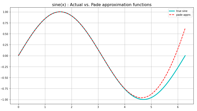
Approximation is a technique that constructs a smooth function which imitates the unknown continuous function by ensuring that the error of approximation is lesser than a certain acceptable upperbound (usually $\varepsilon$) everywhere. Fig 1. shows a Padé approximation for a sine function over a very short interval, already diverging from the desired values past $2\pi/3$. Even a linear approximation as the tangent line to a function is also a locally accurate approximation for most functions, a premise that a lot of system modeling is built on⁴, a classic example of a case where smoothness is not ensured. Thus, any locally linear approach to approximation will require “smoothing” later on to fit the approximation of the true function.

Interpolation on the other hand ensures that the constructed function will pass through certain points called knot points or control points without fail! Knot Points A term commonly used in robot path planning for smooth spline generation⁵, knot points enforce constraints on the smooth curve for the trajectory through space for a robot agent by solving many small boundary value problems where the “boundaries” of individual smooth curves terminate at such knot points.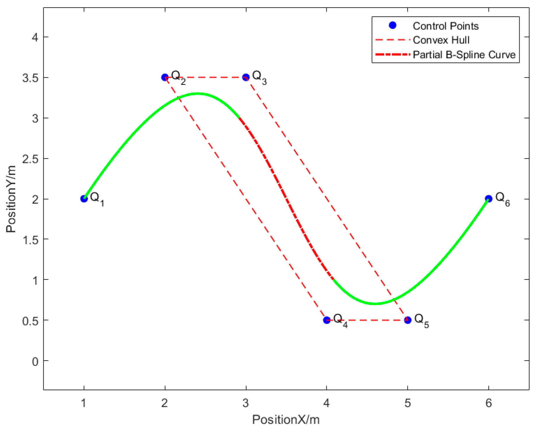

A B-spline based quadrotor trajectory with control (knot) points

And for the cases where discrete samples are available, interpolation is guaranteed to fit a continuous function that will always pass through these discrete sample points while also ensuring smoothness and continuity everywhere.

Whether or not the interpolation function accurately represents the true function in the spaces in between the knot points is a question I hope to address soon as a part of a bigger project, but until then, I will only talk about the construction process itself and limit this article to the implementation of a radial basis kernel function based interpolation along with demonstrations of examples in 1D and 2D.

Radial Basis Functions

Radial Basis functions are popular choices to perform interpolations with. The reason is multifold.

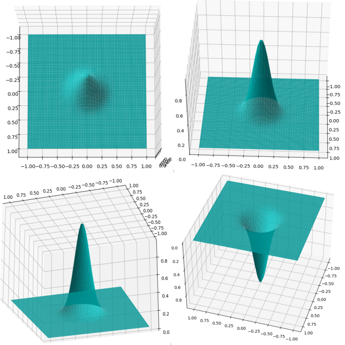
The word radial describes the property of the function as being symmetric about a central axis that is perpendicular to the plane of the function - i.e when viewed from the top or from below. Fig 3. shows an example of a radially symmetric gaussian from different perspectives.

Fig 3. A bivariate gaussian with radial symmetry — **Fig 3.** A bivariate gaussian with radial symmetry

RBF gaussians
Various RBF gaussians with different values of parameter $\varepsilon$ which is inversely proportional to the standard deviation. $Gaussians like in Fig 3. with different values of parameter \varepsilon which is inversely proportional to the standard deviation$

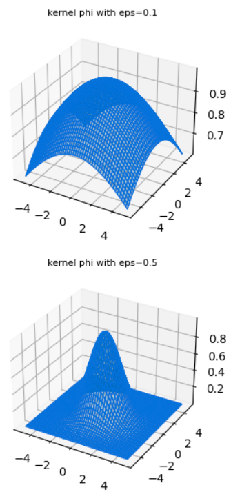
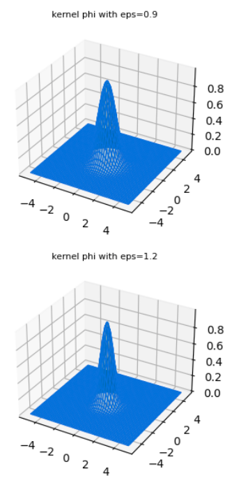
One reason for why they are attractive is because radial symmetry makes these functions rather well behaved, in that they behave predictably in the neighborhood of a point at which they are centered and add homogenously. They have no “orientation” since they are symmetric along all variable axes. And popular choices such as the gaussian basis functions are smooth and differentiable.

A 1D example

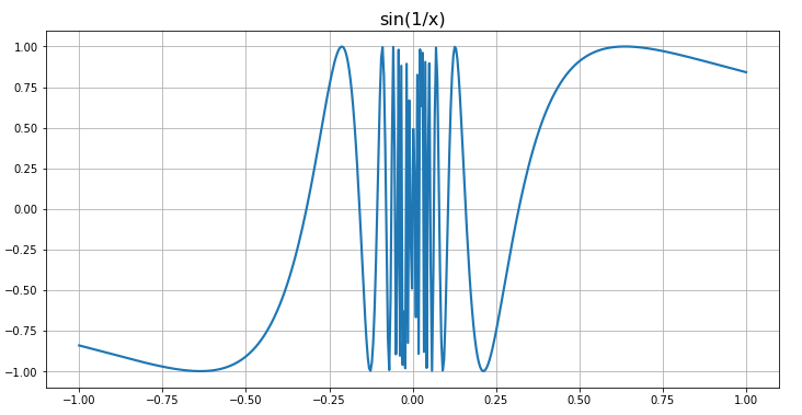
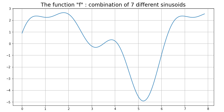
Now I present a 1D example for the interpolation of a true function that we first construct as the weighted sum of sunusoids of different frequencies and phase displacements.

# Number of sample points in the function "f"
N = 500

# The epsilon parameter of the phi() kernel function
eps = 1.5                                  

# The xPts at which the function "f" is originally sampled/spaced
theta = np.linspace(0, 2.5*np.pi, N)

# Array of the 7 frequencies of the 7 sinusoids that are going to be combined
omega = np.array([1, 2, 1, 1, 3, 2, 1])        

# Array of the 7 phase offsets 
phase = np.array([np.pi/5, np.pi/3, -np.pi/4, np.pi/5, np.pi/2, -np.pi/5, -np.pi/3])      

# Initializing the N point vector f
f = np.zeros_like(theta)

# Creating "f" by sequentially adding together 7 sinusoids
for i in range(len(omega)):
    # the frequency omega[i] and with phase displacement phase[i]
    f += np.sin(theta*omega[i] + phase[i])

This produces a very interesting function “f” shown in Fig. 4.

Fig. 4 f a linear combination of 7 sinusoids of different frequencies and phase offsets — **Fig. 4** $f$ a linear combination of 7 sinusoids of different frequencies and phase offsets

Now using a gaussian rbf function modeled as:

\[ \phi(r) = e^{-(\varepsilon r)^2} \]

where $r$ is the point at which the PDF is evaluated Probability Density Function The PDF of a probability distribution is the measure of the likelihood of that sample at which it is evaluated and provides such a relative score to all sample values in the interval of the continuous distribution. and $\varepsilon$ is a quantity inversely proportional to the standard deviation, we perform the interpolation by solving a very simple matrix (linear) equation of the form:

\[B w = f\]

\[ \begin{bmatrix} \phi(||x_0 - x_0||) & \phi(||x_0 - x_1||) & ... & \phi(||x_0 - x_n||)\\ \phi(||x_1 - x_0||) & \phi(||x_1 - x_1||) & ... & \phi(||x_1 - x_n||)\\ \phi(||x_2 - x_0||) & \phi(||x_2 - x_1||) & ... & \phi(||x_2 - x_n||)\\ ...\\ ...\\ \phi(||x_n - x_0||) & \phi(||x_n - x_1||) & ... & \phi(||x_n - x_n||) \end{bmatrix} \begin{bmatrix} w_0\\ w_1\\ w_2\\ ..\\ ..\\ w_n\\ \end{bmatrix} =\begin{bmatrix} f(x_0)\\ f(x_1)\\ f(x_2)\\ ..\\ ..\\ f(x_n)\\ \end{bmatrix} \] for the discrete points $\{ x_0, x_1, x_2 ... x_ \} \in S_x$ sampled from the function $f$.

The leftmost matrix, also called B, or the “interpolation matrix” is constructed by applying the rbf basis function $\phi(.)$ upon the norm of the difference between each sample point $x_i$ with every discrete sample point from $x_0$ to $x_n$. The right hand side is a vector of the true function values at the sample points in order.

The aim is then to “learn” the vector of weights - the vector of values $w_0, w_1, w_2 ... w_n$ such that once solved, we can then interpret the same matrix equation for every single row $\times$ weight vector product as shown below for the 0-th row - a weighted summation of the basis function centered at each $x_i \in S_x$:

\[ \begin{bmatrix} \phi(||x_0-x_0||) & \phi(||x_0-x_1||) & ... & \phi(||x_0-x_n||) \end{bmatrix} \begin{bmatrix} w_0\\ w_1\\ w_2\\ .. \\ w_n \end{bmatrix} = f(x_0) \]

which can be used similarly for any $x_j \notin S_x$ in the domain of $f$ once after the weight vector is solved for as:

\[ w_0 \phi(x_j-x_0) + w_1 \phi(x_j-x_1) + w_2 \phi(x_j-x_2) + ... + w_n \phi(x_j-x_n) = f(x_j)\]

And these weights in the $w$ column vector can be solved for by inverting the interpolation matrix B and multiplying it with the vector of true function values $f(x_i) \hspace{0.2cm} \forall \hspace{0.2cm} x_i \in S_x$ as:

\[ w = B^{-1} f\]

which of course requires that the B interpolation matrix be invertible!

The following snippets of code define functions for the rbf basis and for the interpolation matrix construction:

# define a function for the rbf basis:

def phi(eps, r):
    phi_at_r = np.exp(-(eps*r)**2)
    return phi_at_r



# define a function to make the interpolation matrix

def makePhiMatrix(xPts, kernel, eps):    
    n = len(xPts)                    # number of points in set Sx
    r, c = np.meshgrid(np.arange(n), np.arange(n))
    r    = r.flatten()               # row indices of the B matrix elements
    c    = c.flatten()               # col indices of the B matrix elements
    B = phi(eps, xPts[r]-xPts[c])    # each element in B is phi(eps, x_i-x_j)
    B = B.reshape(n, n)              # reshape n**2 col vector B into a square matrix
    return B

And then the sample points are used to solve for the weight vector $w$:

# Setting up the problem to solve the weights:

# numSamp: number of discrete sample points 
numSamp = 15;      

n = N // numSamp 

# Make a vector of integers - numSamp number of points
sampInd  = np.linspace(0, numSamp*n-1, numSamp).astype(int)

# sample the true function only at the sampInd indices
fSamples = f[sampInd]

# sample the theta values at the same indices
xPts     = theta[sampInd] 

# Make the interpolation "B" matrix
B = makePhiMatrix(xPts, phi, eps)    

# compute he weights
wts = np.linalg.inv(B) @ fSamples.reshape(-1,1)      # w = B_inv @ f

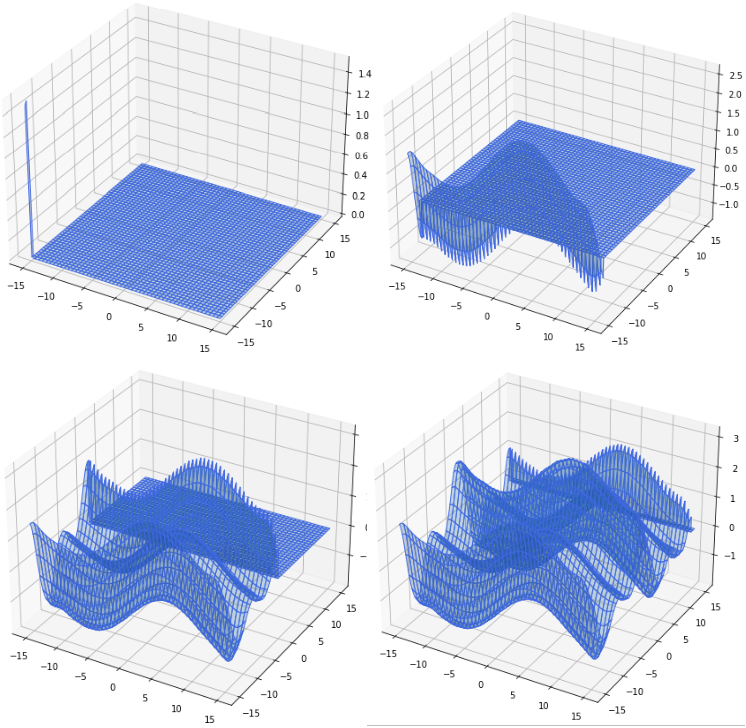
The interpolated function so obtained for different values of the $\varepsilon$ parameter of the rbf gaussian are shown below in Fig. 5

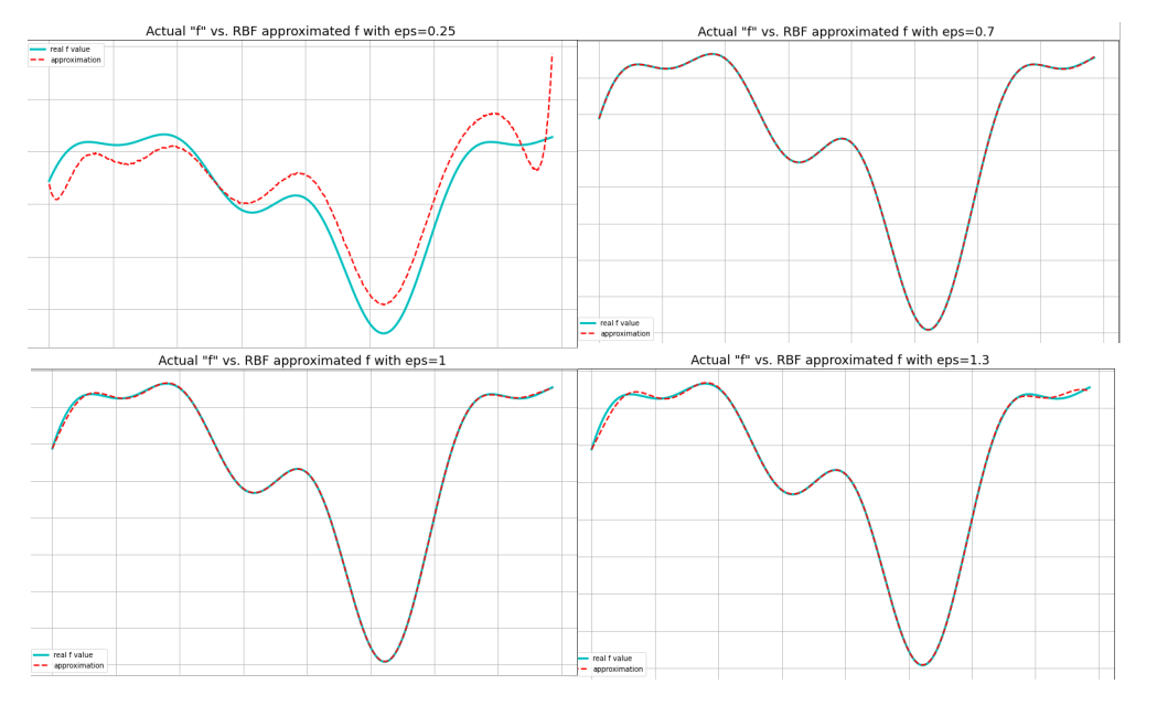
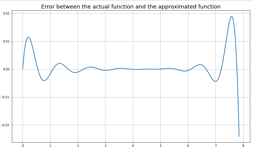
Fig 5. True function f plotted against the interpolated function using rbf bases with different parameter \varepsilon values — **Fig 5.** True function $f$ plotted against the interpolated function using rbf bases with different parameter $\varepsilon$ values

From observation, the best fit was obtained for $\varepsilon$=0.7, the error plot for which is shown in Fig. 6.

Fig. 6 The error, i.e the difference between true f and the interpolated f for the choice of \varepsilon=0.7 — **Fig. 6** The error, i.e the difference between true $f$ and the interpolated $f$ for the choice of $\varepsilon$=0.7

A 2D example

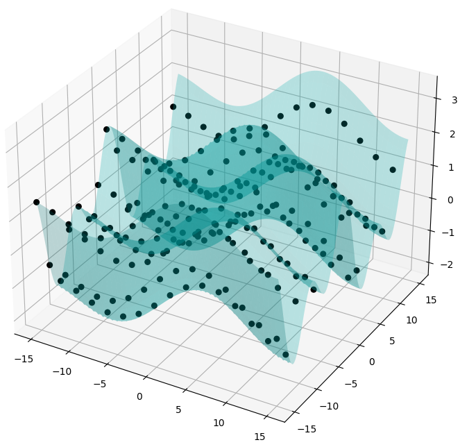
Fig. 7 shows an example of a function in 2 dimensions (bivariate) of the form $z = f(x, y)$ sampled at 225 points in a uniform 15 by $\times$ 15 grid, constructed using an additive combination of independent sinusoids in terms of variables $x$ and $y$:

\[ z = 0.6 \sin(0.3x + \pi/7) + 0.95 \cos(0.8y) + 0.85 \sin(0.085x + 4 \pi/13) + \sin(0.38y + 2\pi/3) \]

$Fig. 7 Sample bivariate function with the 15 \times 15 grid of sample points$

The same construction process as with the 1D case was followed for the rbf based interpolation for the 2D example, described step wise below:

Fig. 8 4 steps of the interpolation process for the 2D interpolation example function shown 500 steps apart — **Fig. 8** 4 steps of the interpolation process for the 2D interpolation example function shown 500 steps apart

The formula for the interpolation (computing the estimated (r_i)) at any point $r_i$ in the domain of the function $f$ is given as: \[ f(x_i) = w_0 \phi(||x_i-x_0||) + w_1 \phi(||x_i-x_1||) + ... + w_n \phi(||x_i-x_n||) \]
This can be read as the sum of points at each of the discrete sampled $x_0$, $x_1$ … $x_n$ points from a gaussian $\phi(r) = e^{-(\varepsilon r)^2}$ centered at $x_i \in S_x$, each term weighted by the corresponding $w_i$ term we solved for.
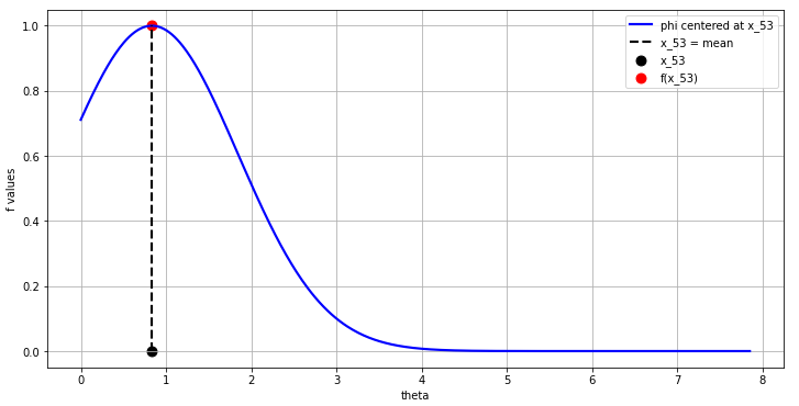
This means that we begin the interpolation at this $x_i$ of interest (this could be anywhere in the domain), let’s say at the 53-rd index value of the 500 point $f$ we were interpolating in our 1D example.
The interpolation at this 53-rd $f[52]$ value begins with the construction of a gaussian with some chosen $\varepsilon$ at this $x_{52}$ value in the domain as shown in Fig. 11:

Fig. 11 The 53^{rd} index value of the domain and a gaussian with \varepsilon=0.6 centered at this sample — **Fig. 11** The $53^{rd}$ index value of the domain and a gaussian with $\varepsilon=0.6$ centered at this sample

Now the values at the set of discrete samples $x_i \in S_x$ are computed along the domain (theta in this example):

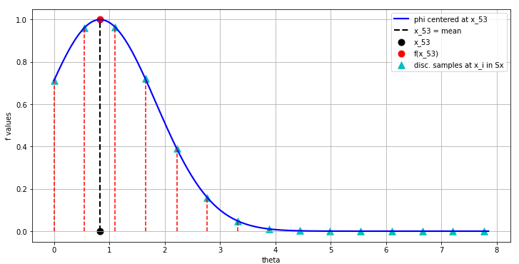
Fig. 12 Discrete samples along the domain from the gaussian centered at x_{52} considered for the interpolation of the f(52) value — **Fig. 12** Discrete samples along the domain from the gaussian centered at $x_{52}$ considered for the interpolation of the $f(52)$ value

Finally, all these blue triangle discrete sample values in Fig. 12 are scaled by the corresponding weights we have precalculated $w_i$ and add them together to produce the single correct value of the the interpolated function at index 52 which matches the original function value $f(52)$ perfectly!

References

Interpolation and Approximation Chapter 2 from urbain.vaes.uk ↩︎
J. M. ain’t a mathematician, Polynomial fitting -how to fit and what is polynomial fitting: https://math.stackexchange.com/q/7129 ↩︎
IIT math notes Chapter 6 ↩︎
Linearization of Nonlinear systems on Collimator.ai ↩︎
Planning Motion Trajectories for Mobile Robots Using Splines, by Christopher Sprunk ↩︎

Radial Basis Function Interpolation

Table of Contents

Interpolating a Function

Radial Basis Functions

A 1D example

A 2D example

References